Spheres in the Nil and Sol geometries
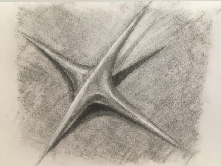 The radius 4 ball in Sol. Drawing: @ Rémi Coulon
In his work on 3-dimensional manifold Thurston proved that there are exactly 8 “geometries” that serve as model for any compact three dimensional manifold. Some of them are familiar to mathematicians, e.g. euclidean, spherical or hyperbolic geometries. Other are rather more exotic.
The Nil and the Sol geometries correspond to the suspension of a torus by a Dehn twist and an Anosov map respectively. The underlying topological space of these two geometries is simply $\mathbb R^3$. However the distance between two points is not the usual one. A natural question is “What is the shape of balls in these geometries?”
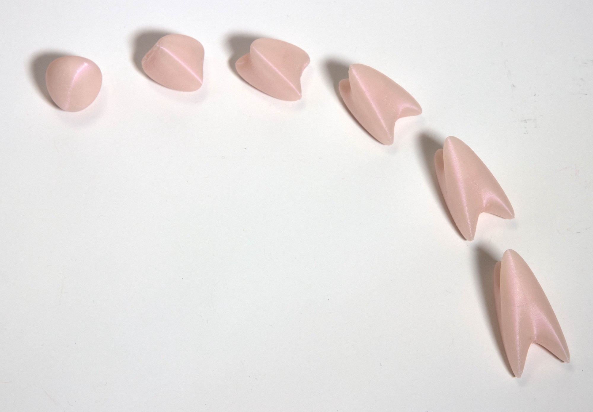
Spheres in Nil
Nil can be represented as the real Heisenberg group, i.e. the set of $3\times 3$-matrices of the form $$ \left( \begin{array}{ccc} 1 & x & z \newline 0 & 1 & y \newline 0 & 0 & 1 \end{array}\right) $$ which we identify with $\mathbb R^3$ through the coordinates $(x,y,z)$. The metric tensor at a point $p = (x,y,z)$ is $$ ds^2 = dx^2 + dy^2 + (dz - xdy)^2 .$$ In this model, one can produce an arc length parametrization of the geodesic flow. In addition one can characterizes which geodesics are globally minimizing distance. This can be used to produce pictures of the spheres of any radius:
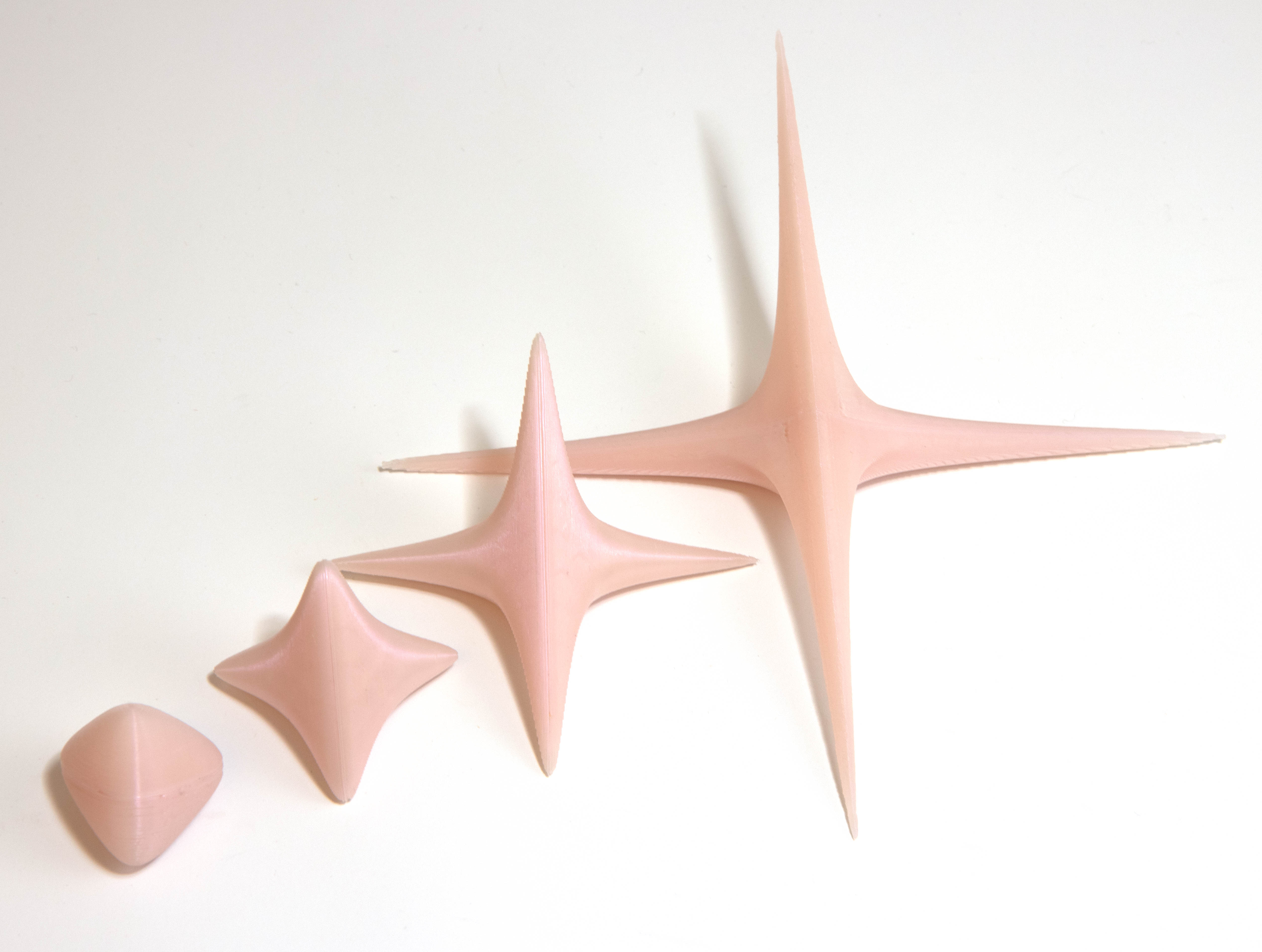
On the picture above, the red curves are the images through the geodesic flow the of the parallels on the unit sphere in the tangent space at the origin. These curves are invariant under the “rotational symmetries” of Nil (which in the Heisenberg model do not match with any Euclidean rotation). The next photo shows 3D printed models of the same balls.
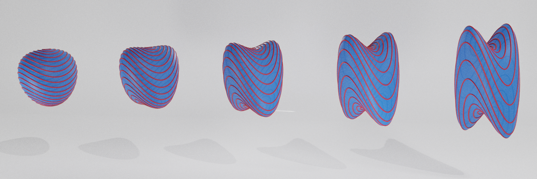
Sphere in Sol
Like Nil, Sol is three-dimensional Lie group. Its underlying space is simply $\mathbb R^3$ while the group law is given by $$(x_1,y_1,z_1) \ast (x_2,y_2,z_2) = (e^{z_1}x_2 + x_1, e^{-z_1}y_2 + y_1, z_1 + z_2)$$ The metric tensor at an arbitrary point $p = (x,y,z)$ is given by $$ ds^2 = e^{-2z}dx^2 + e^{2z}dy^2 + dz^2 $$ This time the geodesic flow is more complicated to integrate. It requires Jacobi’s elliptic and zeta functions. Nevertheless it can be computed numerically. A characterization of globally minimizing geodesics also exists.
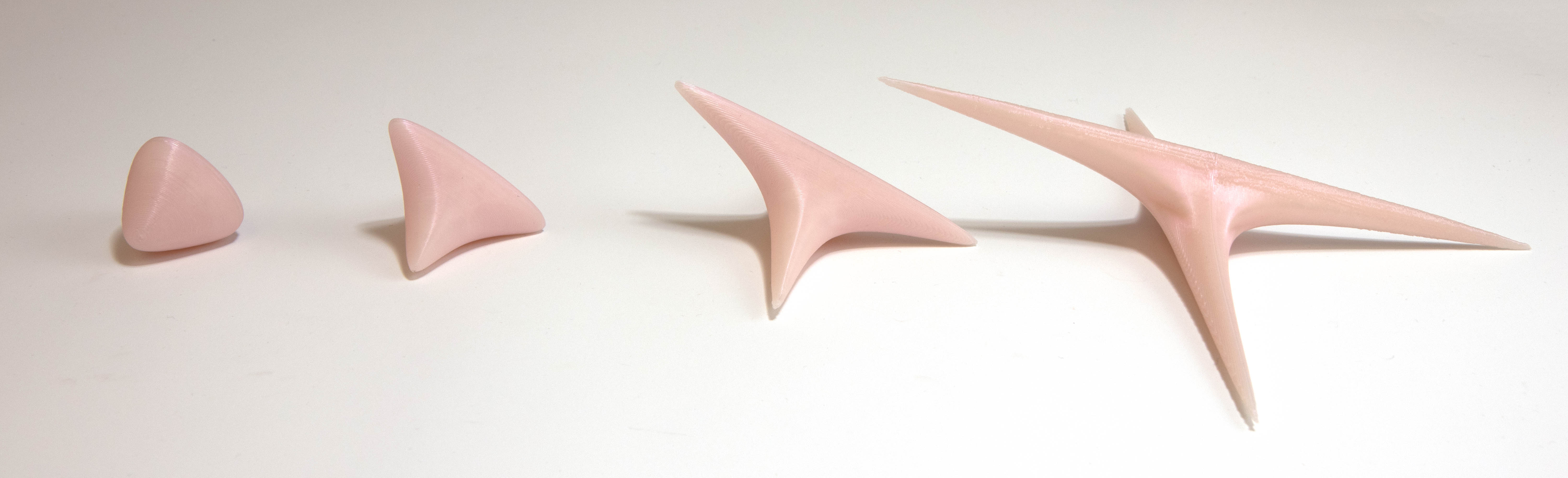
It follows from the exponential weight in front of $dx^2$ and $dy^2$ in the metric tensor that the upper part of the spheres in Sol spreads along the $y$-axis, while the lower part spreads along the $x$-axis. The gallery below shows 3D printed models of the spheres of radius 1, 2, 3, and 4 in Sol
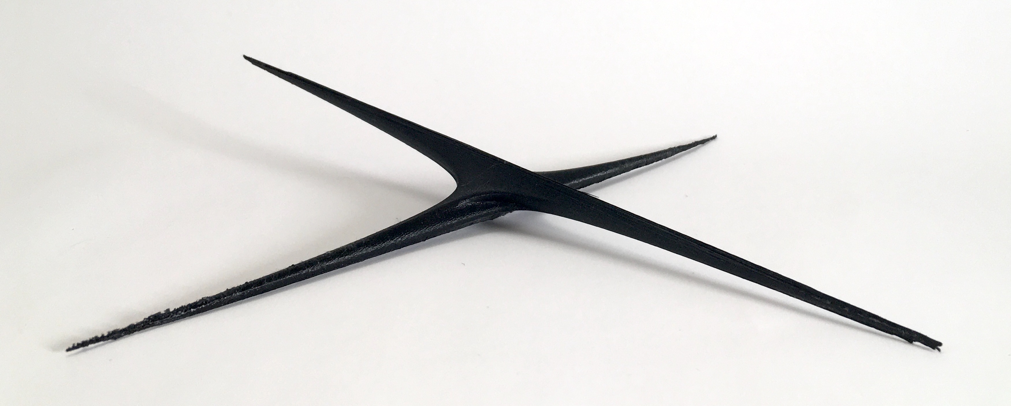
Sol is not uniquely geodesic, i.e. there exist pairs of point $(p,q)$ which are joined by several geodesics. Some are longer that the others. It has the following consequences. The exponential map is not a bijection. Spheres whose radius is larger than $\pi \sqrt 2 \approx 4.44$ are not more smooth. The photos below show a 3D printed model of the sphere of radius 5 in Sol. On can observe a “fold” in middle, which corresponds to the intersection of the sphere with the cut-locus.

To explore the Nil and Sol geometries in virtual, check out this other project