Double Pendulum
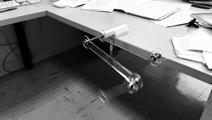 The double pendulum. Image credit: @ Rémi Coulon
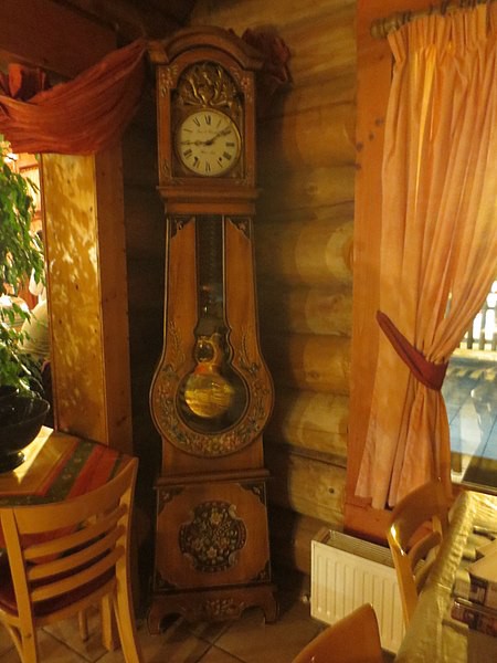
A (single) pendulum is a standard object studied in every mechanics textbook. Its tidy behavior is advantageously used to punctuate grandfather’s clocks.
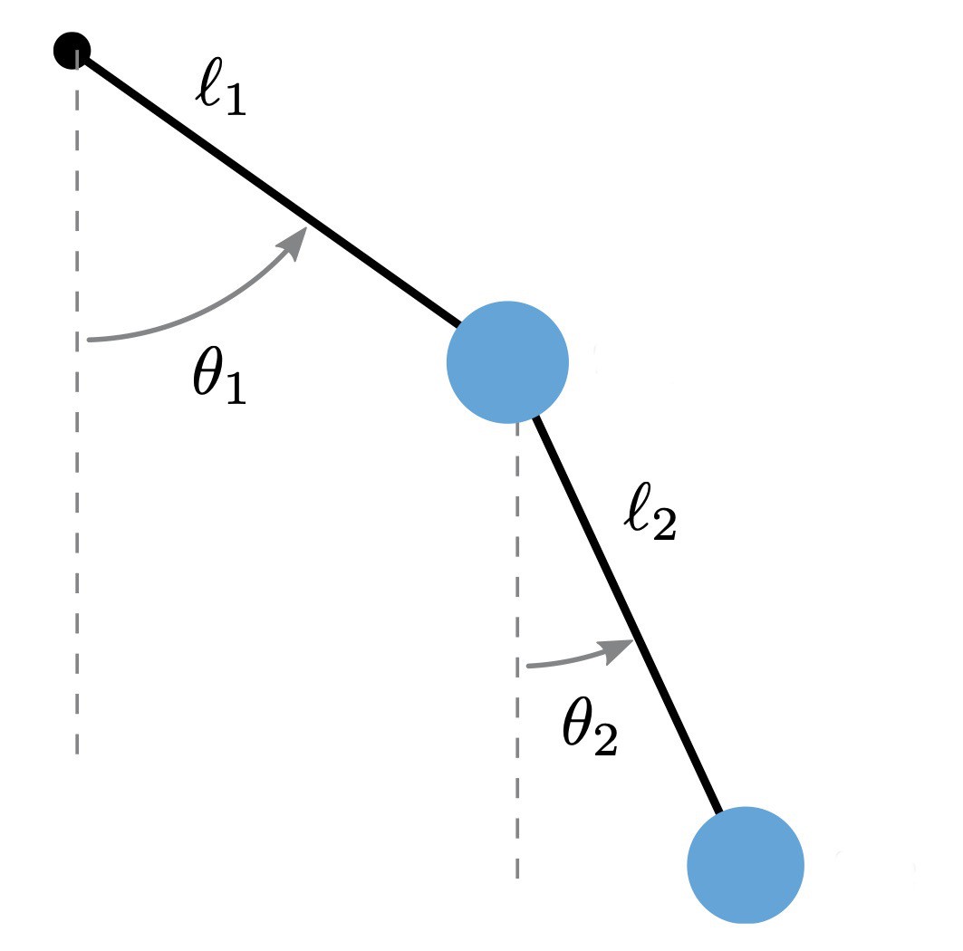
A double Pendulum is a pendulum, with another pendulum attached to its end (see the main picture of this post). Its behavior is much more intriguing. Physically this object can be modeled as follow. We write $m_i$ and $l_i$ for the mass and the length of the $i$-th limb. In addition we denote by $\theta_i$ the angle between the $i$-th limb and the vertical (see figure below).
The laws of physics tell us that $\theta_1$ and $\theta_2$ seen as function of the time $t$ satisfy the following differential equations .
$$\left\{ \begin{split} (m_1+m_2)l_1\ddot{\theta}_1+m_2l_2\ddot{\theta}_2\cos(\theta_1-\theta_2)+m_2l_2\dot{\theta}_2^2\sin(\theta_1-\theta_2)+(m_1+m_2)g\sin(\theta_1)=0 \newline l_1\ddot{\theta}_1\cos(\theta_1-\theta_2)+l_2\ddot{\theta}_2-l_1\dot{\theta}_1^2\sin(\theta_1-\theta_2)+g\sin(\theta_2)=0 \end{split} \right. $$
This system cannot be solved explicitly. Using the Cauchy-Lipschitz Theorem one proves though that for every quadruple $(a_1,a_2,v_1,v_2) \in \mathbb R^4$, there is a unique solution such that $$ \theta_1(0) = a_1, \quad \theta_2(0) = a_2, \quad \dot \theta_1(0) = v_1, \quad \text{and} \quad \dot \theta_2(0) = v_2. $$ Moreover the solution varies smoothly with the initial condition $a_1$, $a_2$, $v_1$ and $v_2$. Smoothly yes, but severly! This system is very sensitive to the initial conditions: two solutions which have close but distinct initial condition will “very quickly” have a totally different behavior. This can be seen on the video below. We launch two copies of the double pendulum with the exact same initial condition (same position, and zero velocity). Exact? Not really. Even the most careful human being will make a small error. This tiny difference induces very different trajectories. This is often referred to as the Butterfly effect .
The “Double double pendulum” on the video was made by Elena Willis during an internship under my supervision at the math department.
The next video is illustrates five different trajectories of the double pendulum, with the same initial position, and slightly different initial velocities.
The picture should be interpreted in the following way. The phase space $X$ of the double pendulum is a $4$-dimensional space: two dimensions for its position given by $\theta_1$ and $\theta_2$ and two dimensions for the velocity represented by $\dot \theta_1$ and $\dot \theta_2$. More precisely each angle $\theta_i$ parametrizes a circle $S^1$. Hence $X$ is the tangent bundle of a $2$-dimensional torus $T = S^1 \times S^1$. However during the motion, the energy of the system is preserved. Hence if $E \colon X \to \mathbb R$ stand for energy functional, each trajectory is contained in a $3$-dimensional subspace $X_c$ of the form $$ X_c = \left\{ x \in X \mid E(x) = c\right\}.$$ It turns out that $X_c$ is a circle bundle over the torus $T$. Indeed the potential energy $V$ of the system is completely determined by its position $(\theta_1, \theta_2)$ on $T$. For such a position, the kinetic energy, which is constrained by $$K(x) = E - V(\theta_1, \theta_2),$$ is a positive definite quadratic form in $\dot \theta_1$ and $\dot \theta_2$. Hence the possible velocities live on an ellipse in the tangent space of $T$ at $(\theta_1, \theta_2)$. In particular, the velocity can be parametrized by a third angle $\alpha \in S^1$.
In order to draw trajectories, we need an embedding of $X_c$ into $\mathbb R^3$. We proceeded as follows. First we chose a level of energy $c$, such that the first limb of the pendulum will never make a complete turn. In other words $\theta_1$ is constrained in the interval $(-\pi , \pi)$. Hence for such an energy level $c$, the possible points in the phase space $X_c$ are completely determined by $$(\theta_1, \theta_2, \alpha) \in (-\pi, \pi) \times S^1 \times S^1$$ which is a thickened torus.
On the video we used this embedding to draw fives trajectories of the double pendulum with the same initial position: $\theta_1 = \theta_2 = 0$. and slightly different velocities, but all with the same energy.